Introduction
MRI stands for Magnetic Resonance Imaging, and it is an imaging technique most commonly used in medical fields. It exploits how nuclei in a strong and constant magnetic field respond when they are “hit” with a weak oscillating magnetic field, such as a radio wave. The way in which the nuclei reacts can be used to measure properties of the material made up of those nuclei. When applied to an object made out of a variety of materials, this technique can be used to contrast the materials to form an image.
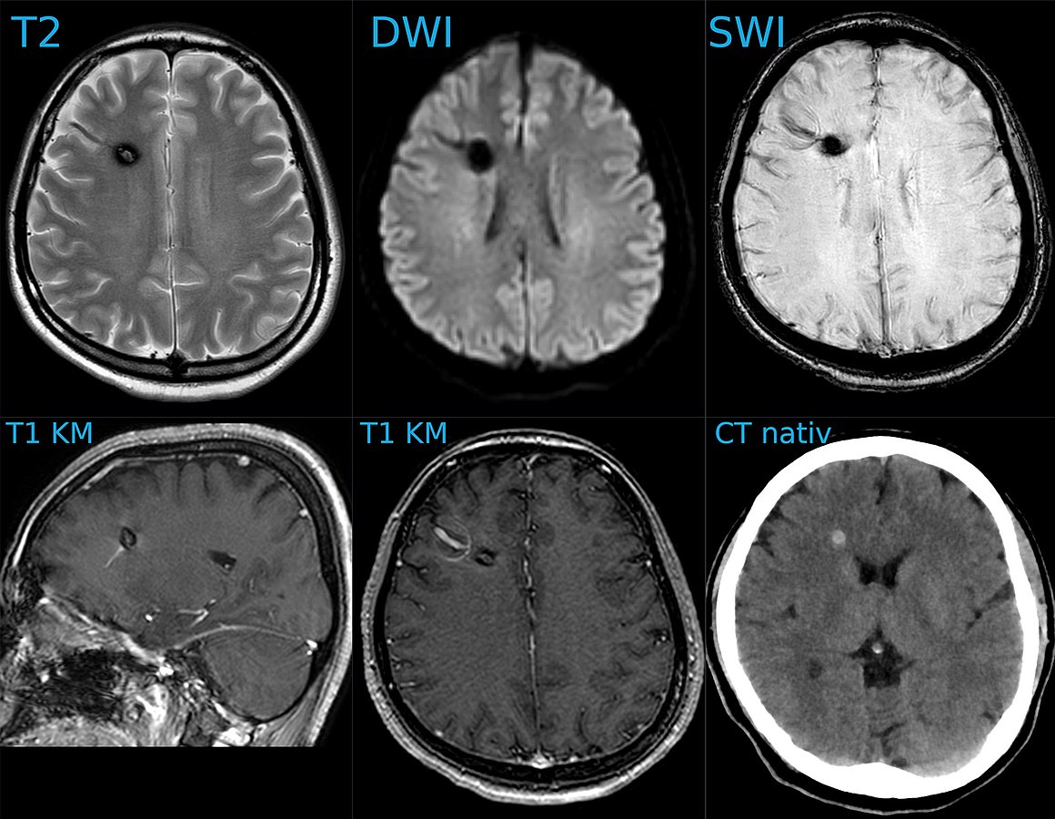
Kavernom und DVA 30W - MR und CT - 001 - Annotation, Hellerhoff, CC BY-SA 4.0 https://creativecommons.org/licenses/by-sa/4.0, via Wikimedia Commons
Uses of MRI
MRI is most commonly used in the medical industry where it is used to provide a cross sectional view of a patient. Its main benefit over other scanning techniques is that it doesn’t require any potentially dangerous forms of radiation, and so it can be a safer way to image a patient - especially if they are likely to need multiple scans over a period of time. Moreover, a radiologist can use a variety of methods for performing MRI scans which can make the scans very versatile to different locations and situations, and so can generally help provide better contrast to make for a better image.
MRI is also useful in many other fields. It can be used to help research in a variety of fields such as geology, plant science, material science, and physics. The ability to study internal structures whilst not destroying them can be incredibly useful when performing experiments. It can also be used in archeology and art history/conservation as it can reveal insights into the history and production of artefacts.
Core Idea
A good initial conceptual mental model for how MRI works is that through using several tricks, we can reliably get protons to send off information about the properties of the structure they are in, and then we can read this information to reconstruct an image. The “core idea” for MRI is in the detail as to how protons send off this information. Let’s start with how to think about a proton. A proton is a positively charged particle with a positive and negative pole. We can then think of it as a bar magnet, and like the bar magnet in a compass it will try and align itself with the direction of any dominant magnetic field. A proton also has a quantum mechanical property called “spin”. Although spin is a quantum phenomenon, we can picture it intuitively as if the proton itself is spinning around its magnetic poles, like how the earth spins around its poles giving us night and day. Your mental model of a proton should look like the following diagram.
proton spinning around poles diagram, Fabien Bryans, This work is licensed under CC BY-NC-SA 4.0 https://creativecommons.org/licenses/by-nc-sa/4.0/
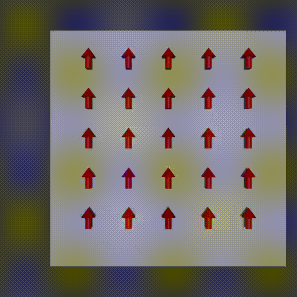
Just like compass needles on Earth, in a strong electromagnetic field you would expect any protons to all align with the field (Note: In practice this doesn’t exactly happen, instead you have some align antiparallel to the field, however you can expect a majority of the protons to align with the field so for all intents and purposes we can just imagine that the protons do all try). However, as the protons are spinning around their poles, when you try and align them in a direction they instead start to precess around the direction you are trying to align them with. You very likely already know what this might look like if you have ever used a spinning top. Gravity wants to align the spinning top but because it is spinning, the top of the spinning top circles around the direction of gravity.
Lucas Vieira, Public domain, via Wikimedia Commons
proton precession diagram, Fabien Bryans, This work is licensed under CC BY-NC-SA 4.0 https://creativecommons.org/licenses/by-nc-sa/4.0/
Now, as a thought exercise and a precursor to what is coming next, imagine if we could put a little coil next to a precessing proton in a larger magnetic field. As the proton is precessing, it means the magnetic field it produces is constantly changing direction. Assuming the coil is positioned upright alongside the proton, then a small magnetic field will be going backwards and forwards sinusoidal through the coil due to the precessing proton. This magnetic field is called the transverse magnetic field. Due to Lenz’s law, this changing magnetic field will induce a voltage in the coil meaning that in this thought experiment we could theoretically read a property of the proton. If the proton had a greater precession angle we would see a larger change in magnetic field in the coil and so a larger voltage. Likewise, a faster precession frequency would see an increase in the rate of change of the magnetic field and so would induce a larger voltage. So, is an MRI machine just a big coil around the patient? Well sort of, but also its not this simple. The reason it’s not this simple is that although this coil example is true for a single proton, you have no guarantee that many adjacent protons will precess in phase with each other (can think of this like dancers who are all facing different directions while they pirouette together). These means the net magnetic field is likely completely cancelled out and so if any signal is induced it would be so minute we would either not be able to detect it or it would tell us nothing.
So how can we get all the protons to precess in phase and then also maximise each proton’s signal? The way we can do this is through creating a perpendicular radiofrequency pulse which is at the same frequency as the proton’s precession frequency (Larmor frequency). This excites some of the protons and means we can view at as if all the poles of the protons become perpendicular to the main magnetic field direction. This means that a larger signal will be induced in the coil. Moreover, the protons will all resonate in phase with the frequency and so will all be in the same phase as each other. This means we can actually pick up the transverse magnetic field for lots of the protons and so we can detect a signal. When the radiofrequency pulse is stopped the protons will de-excite and the signal will disappear. This way of getting a signal is called T2 imaging.
A second way to get a signal is through simply measuring how the protons recover to align with the main magnetic field once the radiofrequency pulse stops. As they align with the field again, the field strength will increase and this can be measured. This way of getting a signal is called T1 imaging.
Understanding T1 and T2 imaging should hopefully show you the “core ideas” which underpin how MRI works. What follows are some further discussions into these imaging types and some of the maths used to model them.
Why Protons?
Why do we always refer to protons and not to some other nucleus? The reason is that a single proton is the nucleus for the Hydrogen atom. Hydrogen is the most abundant type of atom in the human body. The human body is made from about 60% water and as water is made from 2 Hydrogen atoms this hopefully demonstrates why Hydrogen is the obvious atom. Moreover, a Hydrogen nucleus has a high gyromagnetic ratio, which means it will have a faster precession frequency and so can give off a larger signal.
Interestingly, although it is standard for MRI scans to be attuned to Hydrogen, there are times when it can be advantageous for them to be attuned to other atoms. This is due to the idea that protons precess at an angle around their pole. This isn’t how it actually works and instead protons are either in parallel with the field direction or against it. When I talk about changing this angle, I actually mean that a proportion of the protons flip from one state to the other. Every proton which is anti-parallel will cancel out any signal from a proton parallel. Therefore, for a stronger signal you want there to be a large difference in the number of protons in the parallel and anti-parallel state. For clinical MRI, this number is actually surprisingly low at only a difference of a few protons for each one million protons. A technique called hyperpolarisation can be used to increase this difference and get much better imaging. Common gasses included Helium-3 and Xeon-129. These are both noble gases too and so can be safely inhaled by humans. They can therefore be used to image the gas space such as for lungs in much higher fidelity.
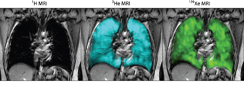
Figure 2. Conventional 1H MRI, hyperpolarised 3He and 129Xe MRI, Kirby et al. “Pulmonary functional magnetic resonance imaging for paediatric lung disease.”, Paediatric respiratory reviews 14 3 (2013): 180-9
T1
The T1 signal is defined by the equation:
$$S(t) = M_{0}(1 – e^{-t/T1})$$
Where M₀ is the Boltzmann magnetization of the sample. This is the maximum amount of longitudinal magnetization from the sample which will be when none of the protons are excited.
If you are familiar with electronics, you will notice this is in the same form as the equation for charge on a capacitor over time after discharge. When picking a value of t (for T1 its referred to as the repetition time, or TR value) you will get the highest signal when picking a large value, however this will make the scan itself take much longer and also depending on the materials may mean you lose contrast. T1 relaxation takes longer (at a maximum over 2000 ms) than T2 relaxation (at a maximum of about 140 ms).
Although having a long TR value can help with getting a larger signal from the T2 scan because it means you are waiting longer between T2 scans and so more protons will be susceptible again to the radiofrequency pulse and so you will get a stronger initial transverse signal which should help for a T2 scan.

© Nevit Dilmen, CC BY-SA 3.0 https://creativecommons.org/licenses/by-sa/3.0, via Wikimedia Commons
T2
A T2 weighted scan is slightly more complicated to derive its signal equation. If the transverse magnetic field is sin(ωt) where ω is the precession frequency of the proton, then due to Lenz’s law being the rate of change of magnetic field the signal received will be ω ⋅ cos(ωt). In addition, the strength of the signal will scale with the number of protons, N. It will also scale sinusoidal with the angle of precession, θ. Therefore, the signal should be:
$$sin(\theta) \cdot N \cdot \omega \cdot cos(\omega t)$$
However, remember that the angle of precession, θ, will decay after the excitation pulse has been applied. This means it is more accurately represented as an additional free induction decay of e^(-t/c1) for a constant c1. Additionally, as the proton lose coherence with each other, due to their own magnetic fields mildly affecting each other, we would expect this whole transverse signal to decay too. This can be modelled as a free induction decay term of e^(-t/c2), for some constant c2. The signal equation therefore is:
$$ \begin{align} &e^{\frac{-t}{c1}} \cdot N \cdot \omega \cdot cos(\omega t) \cdot e^{\frac{-t}{c2}} \nonumber \\ \implies &N \cdot \omega \cdot cos(\omega t) \cdot e^{\frac{-2t}{c1+c2}} \nonumber \\ \implies &N \cdot \omega \cdot cos(\omega t) \cdot e^{\frac{-t}{\frac{1}{2}(c1+c2)}} \nonumber \\ \implies &N \cdot \omega \cdot cos(\omega t) \cdot e^{\frac{-t}{T2}} \nonumber \\ \implies &A \cdot cos(\omega t) \cdot e^{\frac{-t}{T2}} \nonumber \\ \end{align} $$For a constant, A, which corresponds to starting signal strength (will be higher for a longer TR value)
Deciding when to measure t (referred to as the echo time, or TE) depends on how to get the best contrast between the materials. However, in general picking a low TE time will give you the most signal before it dies out.
Afiller at English Wikipedia, CC BY-SA 3.0 https://creativecommons.org/licenses/by-sa/3.0, via Wikimedia Commons
If you were to try T2 imaging in practice though, you would notice that the signal decays much quicker than expected. Why is this? Well, a core assumption about T2 imaging is that the protons are all feeling the same magnetic field strength. In practice, there will be a slight gradient in the magnetic field strength across the area being measured. This means that the protons in a stronger part of the magnetic field will have a slight higher ω and so will gain phase quicker, and those in a weaker part will have a lower ω so will lose phase quicker. The result is that the free induction decay is much quicker than expected. This new decay rate is referred to as T2*, and is as follows:
$$\frac{1}{T2*} = \frac{1}{T2} + \gamma \cdot \Delta \Beta$$
Where γ is the gyromagnetic ratio, and ΔΒ is the change in magnetic field strength over the area.
This is a problem as it means that getting a high-fidelity scan is much harder as we lose signal faster. There is however a clever way to mitigate the change in magnetic field strength by using the spin echo.
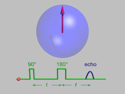
The Spin Echo
The spin echo is quite a simple idea. Basically after τ amount of time, the protons will have de-phased by some function, ƒ(τ, ΔΒ). For any fixed τ, this function is an odd function as for every positive and negative ΔΒ pair, they will have de-phased by the same magnitude, just in different directions. We can use this idea to use another radiofrequency pulse to make all the protons be in phase again after an echo period.
To do this, we need to use a radiofrequency pulse at time τ, and 180 degrees to the original pulse. This will make the direction of precession reverse and so after another τ seconds, we will see all the phases align again giving us the perfect opportunity to take a high signal reading as the T2* constant becomes T2.
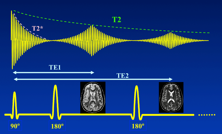
A double-echo SE sequence, Courtesy of Allen D. Elster, MRIquestions.com
Above you can see what the signal magnitude looks like for a τ of TE1/2 seconds.
Hahn Echo, Gavin Morley, CC BY-SA 3.0 https://creativecommons.org/licenses/by-sa/3.0, via Wikimedia Commons
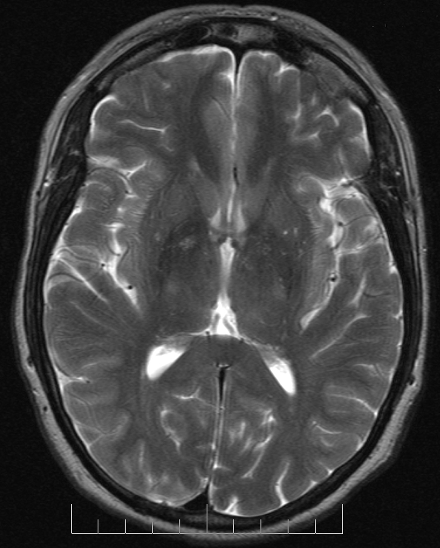
Spin Density Imaging
Spin density imaging is another form of imaging where you use a long TR time and an almost immediate TE time. This means that you basically read the following signal at time t=0:
$$N \cdot \omega \cdot cos(\omega t) \cdot e^\frac{-t}{T2}$$
Which if t=0, is just N · ω.
Assuming ω is the same across all the protons, this gives us a signal which scales with the number of protons. Therefore, we now have a way of getting the density of the protons, which is referred to as the spin density scan.
Figure 8. Proton density axial brain image, Paschal and Morris, “K-space in the clinic”, J. Magn. Reson. Imaging 19 (2004): 145-159
Location and Imaging
Overview
We now understand how to get a signal from a large group of protons. However, you may still have many questions about how MRI scans are actually produced. How do we use these signals to image the protons in the sample? How can we spatially localise a signal? How do we ignore protons we don’t want to image?
The main idea about how we actually image a sample is that instead of imaging it like with pixels from a camera, we take several readings which we perform operations on and combine to reconstruct the image. We introduce a magnetic field gradient across the sample and then use this added information to be able to spatially differentiate signals.
Fourier Transforms
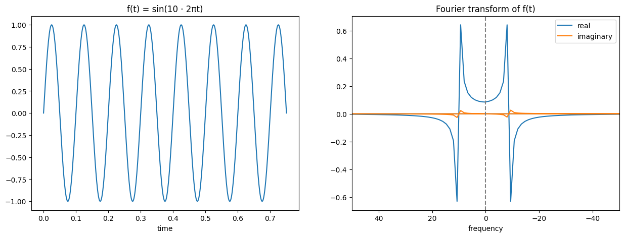
Probably the most important thing to understand for MRI imaging is the Fourier transform. I won’t go into too much detail, but the idea of a Fourier transform is that it converts a signal from the time domain the frequency domain. If you consider a sine wave (below left), you can see how this is a wave of a constant frequency and so we could represent it on a graph of amplitude and frequency (below right).
This example seems too obvious though, surely there are only a few functions which can be converted to a combination of sine waves of differing frequency and amplitude (and phase)? However, the Fourier series shows us how we can do this for most functions we would want to use. We can use the Fourier transform as an operation to perform this conversion. The Fourier transform is expressed below:
$$F(\omega) = \int^{\infty}_{-\infty} f(t) \cdot e^{- i \omega t} dt$$
As said, I won’t be going into detail on this or how it works, but I will try and help build some intuition of how to view it. You might have noticed that the Fourier transform of a sine wave earlier had blue and orange lines, why did it need multiple colours? The reason is that it produced complex outputs and so each real value actually has a corresponding imaginary part. This imaginary part is expressed by the orange colour, while the blue colour expresses the real. The way to read this is that for the transformed function, the new x coordinate is the frequency of the sine wave (i.e. further away from the origin will represent a high frequency sine wave, close to the origin a low frequency wave), the real part’s y coordinate (blue) represents the amplitude corresponding to that sine wave frequency, and the imaginary part’s y coordinate (orange) represents the phase shift corresponding to that sine wave frequency.
Here are some other examples to hopefully help build intuition and understanding:
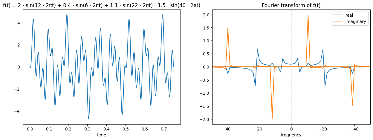
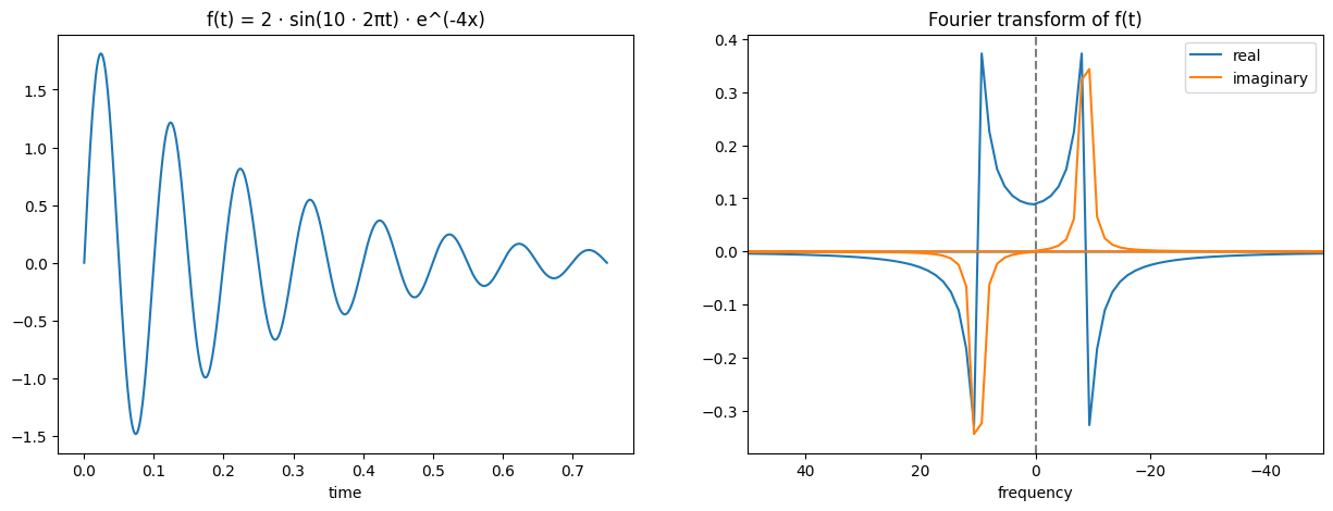
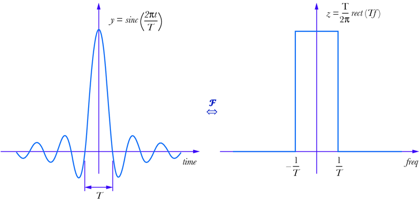
Figure. 8: Fourier transform of a sinc function, Huageng Luo, “Physics-based data analysis for wind turbine condition monitoring” (2017), CC BY-NC 4.0 https://creativecommons.org/licenses/by-nc/4.0/
I said earlier that the Fourier transform converts between the time domain and the frequency domain, but it doesn’t actually have to be the time domain. For example, it could be the space domain. A space domain signal could be something like light diffraction patterns where you have peaks and troughs. You can see how this sort of looks like a sine wave, but instead of the x axis measuring time it would measure space.

Diffraction sunlight - color channels, Pieter Kuiper, Public domain, via Wikimedia Commons
For more depth into the Fourier transform, you can check out 3blue1brown’s video on it, the Wikipedia page, or maybe I’ll even make a blog article about it! It’s a very useful tool with applications in many fields!
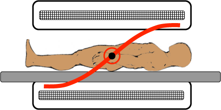
Slice Selection
Let’s approach one of the first problems, how do we ignore the protons we don’t want to get a signal from? If you imagine a human lying in an MRI machine, if you were to send in a radiofrequency pulse it would excite all of their protons and so when you tried to read back a signal it would be from the whole human. What would be more helpful would be if you could just excite a specific centimetre slice of a human as this could be reconstructed into a 2D image. Fortunately, there is a way to do this!
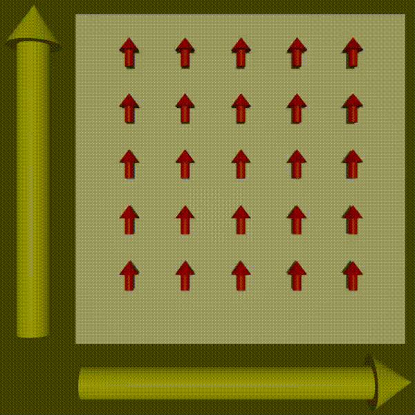
Before you send in a radiofrequency pulse, you turn on magnets to produce another magnetic field across the patient, however this field is not constant across them and is instead a gradient meaning that the field strength will gradually change as you move down the patient. This means that the protons at the head of a patient will be in a stronger magnetic field than the protons in their feet. As such, the precession frequency of their head protons will be higher than their feet protons. Therefore, if you send in a radiofrequency pulse attuned to the frequency of their head protons, it will excite them without exciting the feet protons.
Gradient linearity, Courtesy of Allen D. Elster, MRIquestions.com
So, can you simply do this for a specific centimetre slice? Unfortunately, if you send in a pulse with the a frequency at the middle of the slice, it will excite too few protons due to it being such a specific frequency. Instead, what you need to do is send in a pulse which excites all frequencies covered by that slice and no more. How do you do this?
We can rephrase this question to help us solve it. How can we construct a signal which is created from exactly a specific continuous range of frequencies all at the same amplitude? This is just the inverse Fourier transform of a square range, and we’ve even seen the example of it earlier.
Figure. 8: Fourier transform of a sinc function, Huageng Luo, “Physics-based data analysis for wind turbine condition monitoring” (2017), CC BY-NC 4.0 https://creativecommons.org/licenses/by-nc/4.0/
Therefore, we send a radiofrequency pulse of the sinc wave (left above) to excite that very specific band of frequencies and so equally excite across the slice we want and no further. That is how we do slice selection! This slice can be chosen as any plane across the 3 axes.
Frequency Encoding
At this point we have only the desired slice’s protons excited and spinning in the transverse plane. If we took a reading, we would see the signal from all of this plane, so how can we differentiate protons spatially now? Frequency encoding is one method for doing this. It works by applying a magnetic field gradient across the slice and so protons at different points along the gradient will have different transverse frequencies. When you then take a reading of the produced signal it is the sum of these different frequencies. By using a Fourier transform, you can pick out the contributions (amplitude and phase) made by each frequency. This will now give you information on each column of the slice.
frequency encoding diagram, Fabien Bryans, This work is licensed under CC BY-NC-SA 4.0 https://creativecommons.org/licenses/by-nc-sa/4.0/
Back Projection
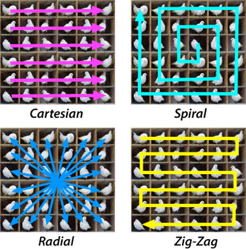
Using just slice selection and frequency encoding, we can actually now image a sample. You do this by doing a frequency encoding, taking a signal, and then rotating the sample and repeating. Once you have done this for the full rotation of the sample, if you combine all the data points you can reconstruct an image. This was one of the very early methods of MRI and is known as back projection. However, back projection can often have many aliasing artefacts and the resultant image is usually sampled a lot at the centre but lacks a lot of visual clarity towards the edges. Therefore, backprojection is not an ideal imaging technique to use.
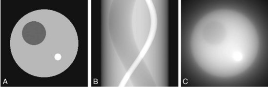
Figure 16-6. Computer-simulation phantom used for testing reconstruction algorithms (Computer simulations performed by Dr. Andrew Goertzen, University of Manitoba, Canada), Tomographic Reconstruction in Nuclear Medicine, Radiology Key
K-Space
To understand a better way of imaging a slice, we first will need to understand K-space. K-space is the resulting 2D discrete Fourier transform of a discrete 2D input. Every pixel in K-space has two values, a real amplitude and an imaginary phase.
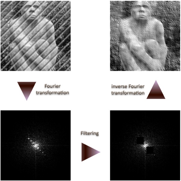
Fourier filtering, Devcore, CC0, via Wikimedia Commons
The way you get to K-space is you first do a Fourier transform for each column, and then you do a Fourier transform on each row of the result. You can read K-space by viewing every coordinate as a phasor corresponding to a unique 2d sinusoid (like a wave) which has an angle and frequency based on the phasors position in K-space, and an amplitude and phase based on the real and imaginary parts of that phasor in K-space. This is why in many K-space images the centre is bright (a high amplitude value). This is because the central pixel corresponds to a wave with a very low frequency, meaning that it effectively is the contribution of a minimum/base value to the whole of the image.

2D Fourier Transform and Base Images, Felix Lugauer and Jens Wetzl, CC BY 4.0 https://creativecommons.org/licenses/by/4.0, via Wikimedia Commons
If you have ever heard of high pass or low pass filters, you can digitally create them for images using a 2D Fourier transform, an operation to apply the filter, and then the inverse 2D Fourier transform. For example, if you want to do a high pass filter and remove the low frequency components of an image you can set all values less than some distance from the centre to 0, and then do an inverse Fourier transform and get the image without the low frequencies. This image has detailed more defined making it better for some image processing tasks such as edge detection. A low pass filter is the same procedure but setting all values to 0 which are outside some distance from the centre. A low pass filtered image will lack detail but will maintain general shapes and patterns of the image, because of this it can be used as a technique for lossy compression.
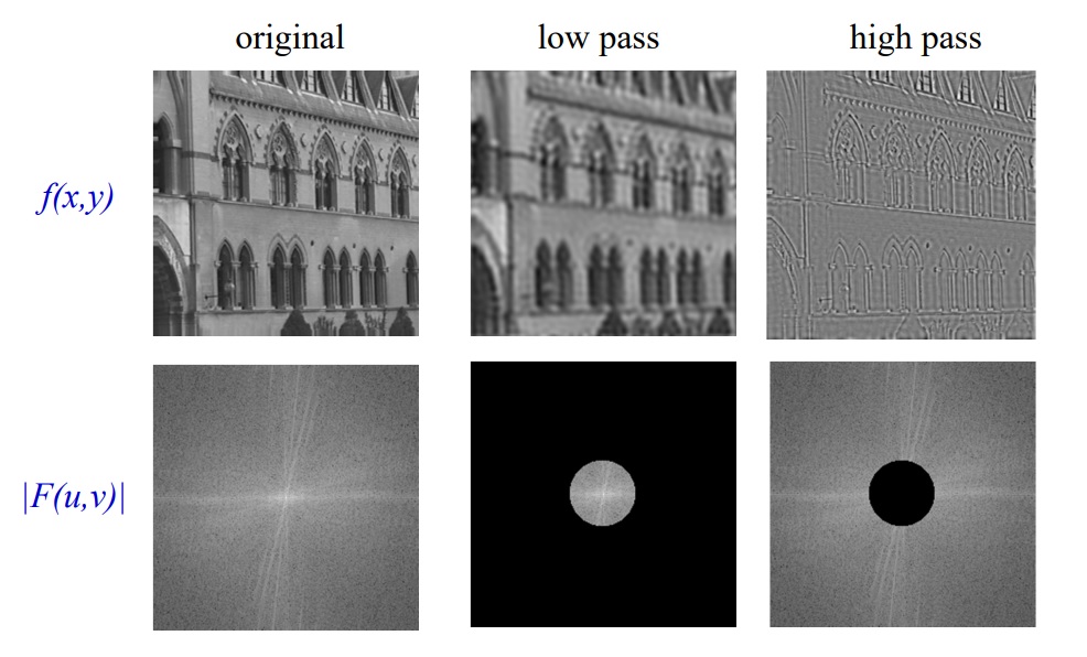
Example: action of filters on a real image, A. Zisserman, B14 Image Analysis; Lecture 2: 2D Fourier transforms and applications
The main thing you need to be aware of is that K-space is a 2D encoding of 2D spatial frequencies, and that the location of each K-space phasor corresponds to the contribution made by a 2D sine wave.
Phase Encoding
So, with frequency encoding we could apply a magnetic field so that we could determine column values along one dimension. The idea with phase encoding is that it’s a second way to encode positions and so you can use it orthogonally to frequency encoding to be able to pick out signal values from every x,y coordinate pair.
The way it works is similar to frequency encoding. You apply a magnetic field gradient over a distance and so the protons where the field is stronger spin faster, and where it is weaker spin slower. You turn this field off shortly after starting it though. The result is that along that direction all the protons return to the original precession frequency, however they are now at different phases from each other as a result from the temporary speed up.
phase encoding diagram, Fabien Bryans, This work is licensed under CC BY-NC-SA 4.0 https://creativecommons.org/licenses/by-nc-sa/4.0/
Used in combination with frequency encoding you have now encoded information to be able to pick up row and column frequencies and so the signal can be used to construct a K-space of what you are scanning, and so you just need to do the inverse to get the original image back. For more intuition of this working, observer what happens to the phases of the protons as you apply two gradients.
k-space encoding diagram, Fabien Bryans, This work is licensed under CC BY-NC-SA 4.0 https://creativecommons.org/licenses/by-nc-sa/4.0/
You can see how this corresponds to a wave pattern, i.e. a point in K-space. Therefore, you can use the resulting MRI signal to determine the amplitude and phase of the phasor. By moving around and measuring in K-space you can get enough information to produce the K-space of the slice and then to get the image you just do the inverse Fourier transform!
Scanning Procedures
The most common scanning procedure is called The Gradient Recalled Echo Sequence. We have now covered all the parts of it so that you should be able to understand it.
The first step is to create a gradient so that you can do slice selection. Once you have created this gradient, you then send in a radiofrequency pulse like a sinc wave to work with the slice selection gradient to excite just that slice. Next you encode phases within the resulting slice (lets say x, y plane) to get the phases positioned so that you can read a row of K-space. This means you need to get to kx, ky and then you turn off the phase encoding gradients and turn on the frequency encoding gradient to move across all of kx for a fixed ky (assuming the frequency encoding gradient is along the x axis). As you do this you note the signal received through an analogue to digital converter (ADC). You do this changing the initial K-space starting position each time by using a different phase encoding gradient (in this example in the y axis). Each row of K-space will take time TR to collect. After you have done this for each row of K-space you have got enough data to create K-space and form an image for the slice. If you want a 3D scan, then you just repeat this for different locations in slice selection to get multiple layers.
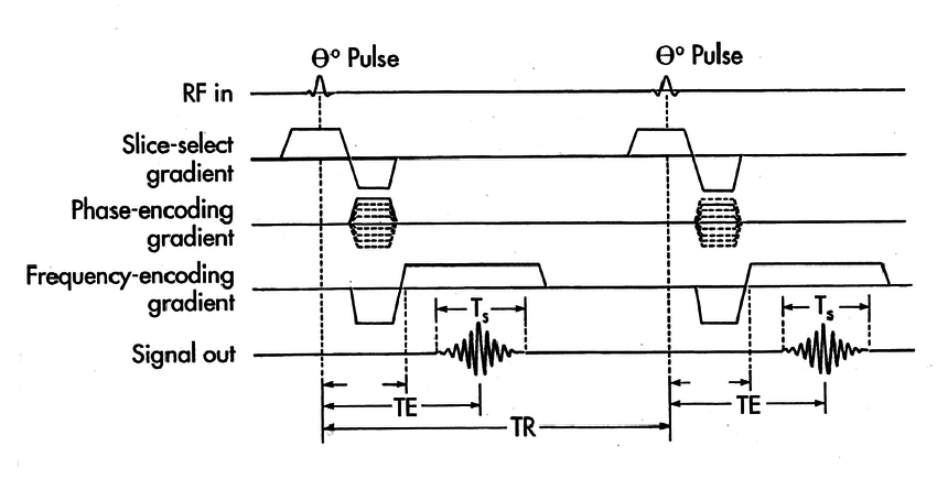
Figure 4. 2D gradient-echo pulse sequence diagram, R. Edward Hendrick, “Breast MRI: Using Physics to Maximize Its Sensitivity and Specificity to Breast Cancer”
There are a couple of things to note here. Firstly, the slice selection gradient is inverted and played for half the time it is played positively after the radiofrequency sinc pulse finishes. This is because the sinc pulse excites protons along the slice at different rates meaning that they are not in phase with each other straight after all of them being excited. This can be solved by just applying the gradient backwards for half the time it was on to reverse the phase loss so that they are all in phase (similar in some ways to the spin echo). Secondly, note that the phase gradient is the only thing which changes between each cycle making up a slice scan. This is because you need each cycle to start at a different point in phase space. You can make the scan faster but the sequence slightly more complicated by using something called echo planar imaging where you cover K-space in a more efficient way using both x and y phase encodings to do a snake like pattern meaning there is less downtime from the phase encoding.
Methods for filling k-space, Courtesy of Allen D. Elster, MRIquestions.com
Scanner structure
The MRI scanner is made up of 3 main components: a main magnetic coil, a set of gradient coils, a radiofrequency coil.
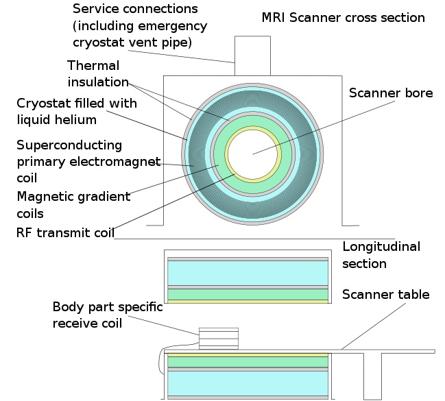
Mri scanner schematic labelled, CC BY-SA 3.0 https://creativecommons.org/licenses/by-sa/3.0, via Wikimedia Commons
The main magnetic coil’s job it to provide a strong, homogeneous magnetic field (Β₀ field) over the patient so that all the protons have the same high procession frequency. The strength of the field is dependent on the amount of current going through the coil – the more current the higher the field strength. However, this causes higher resistance and heat and so could be unsafe. This problem is solved by using a superconducting material which has no resistance at a low temperature. This coil is therefore in contact with liquid Helium to ensure it remains at a temperature of less than a few Kelvin so that we can have a higher current and field strength. This magnetic field strength is often on the order of 1 Tesla, with 1.5 Teslas being a common MRI machine strength. Very small changes in the magnetic field strength can lead to signal problems which is partly why the magnet is so large. Despite this, there will be inhomogeneity in the field but the centre of the scanner will usually be the part of the field with the least change. This point is known as the isocentre and is the best area to take scans from.
The gradient coils provide smaller magnetic gradients so that you can do slice selection, gradient encoding, and frequency encoding. You will usually have a gradient coil for the x, y, and z direction. They can be used in combination to create slices at different angles. The magnitude of the field strength of these coils is on the order of a few Milliteslas.
The radiofrequency coil will create an excitation radiofrequency pulse to flip protons and may also be used for reading the transverse signal from the protons (although in practice you may use another coil closer to the patient). The RF coil will transmit these pulses by varying in time a magnetic field of the order of Microteslas. Remember that the pulse from the RF coil will affect the whole patient and it is not the mechanism we use to excite only a specific part of the patient.
Summary
MRI is an immensely useful imaging technique which can safely provide insights to help with diagnosis and further treatment. Hopefully this article has given you a clearer understanding of why and how it works. Please keep in mind that “MRI” is a massive field and covers a wide variety of methodologies and tricks to improve imaging and so although this guide has covered the basics, there is so much more to learn!
Further resources
There are many excellent resources to learn more about MRI and to see different explanations of what has been discussed here. If you want a great in-depth understanding of the basics, I can really recommend thePIRL’s “How MRI Works” playlist - it provides some amazing visualisation to help demonstrate what is going on. Other video recommendations include Radiology Tutorials’ “MRI physics course” which provides many details in lots of areas. For a quick video going over the whole process, I can recommend Doctor Klioze’s video called “MRI: Basic Physics & a Brief History”.
For text and articles on the topic, I have two recommendations. Firstly is Wikipedia, which seems to have pretty good literature on MRI. It can be especially useful to find out more about the details about the maths. My other recommendation is MRI questions, from which several of the diagrams in this article are from. MRI questions covers the field quite widely in nice bite-sized articles which will often include many good diagrams.