What is the Markov inequality
Below is the formula for the markov inequality. Don’t worry about understanding it yet, just know that you can refer back to it here.
$$P(X \geq a) \leq \frac{E(X)}{a}$$
The markov inequality gives us a gaurantee about any distribution where samples of the distribution are all non-negative. Using the Markov distribution we can determine an upper bound on the probability of a sample being above some other value. For example, let’s consider the distribution of the lengths of baguettes produced in a bakery. We might not know much about this distribution. We might only know the average length of a produced baguette and nothing more. If we couldn’t determine what distribution fits this, how would we answer the question of what is the probability that a baguette is longer than 80cm? Given we are certain of the mean length, we can use the Markov inequality to provide an upper bound on the probability of this.
Let’s say the average is 65cm. Then the Markov inequality tells us the probabilty is no higher than 65/80 = 0.81. If we consider any other distribution we can know for certain that it will not give a probability higher than this. For example if the distribution is actually a normal distribution with a standard deviation of 10, then the probability of a baguette being longer than 80cm would be 0.07. If it was a uniform distribution between 35 and 95, then the probability would be 0.25. Regardless of the distribution used, we could gaurantee it would be less than 0.81 because of the Markov inequality.
A fair response to this would be - “but that doesn’t seem like a very good bound”. While true, the gaurantee it gives us (even though we know so little about the distribution) is why it’s useful. This is why the Markov inequality is used in many proofs as it can provide some gaurantee/target which needs to be met for a property to hold for an arbitrary distribution. An interesting related question to the first response would be - “why is it such a bad bound?”.
Worst case example
To answer the question of “why is it such a bad bound?”, let’s instead ask the question - “what is the distriubtion where this worst case bound would be exactly correct?”. Remember, the Markov inequality works for any arbitrary distribution so long as it is non-negative. Therefore, we can construct whatever distribution we want as long as it doesn’t have any negative values and has a mean of 65cm. If we start by acknowledging that some distribution should exist where the probabilty of 80cm is 0.81, then we have only 0.19 worth of “probability” left to assign. We have the constraint that we need the average to be 65cm, so if we try with a distribution where the probability of creating an infintesely small baguette is 0.19, then we can meet this constraint.

$$80cm \times 0.81 + 0cm \times 0.19 = 65cm$$
Note how there would be no way we could get the average lower without creating a distribution where we can produce negatively long baguettes.
Intuitively deriving the Markov inequality
A seesaw is a board with a pivot at some point along the board, usually in the middle.
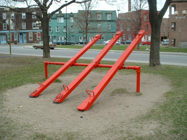
A Seesaw in a park in Montreal, photographed by aarchiba, Public domain, via Wikimedia Commons
In a playground you’ll see one person sit on one end and another person on the other. We can tell which way the seesaw will rotate round its pivot if given pairs corresponding to people’s weights and their distance from the pivot. You simply calculate the clockwise and anti-clockwise moment and for whichever is bigger, it will rotate in that direction. The clockwise moment of the seesaw will be the sum of weight x distance from the pivot for all the people on the right hand side of the pivot. If the clockwise and anti-clockwise moments are the same then the seesaw will remain balanced.
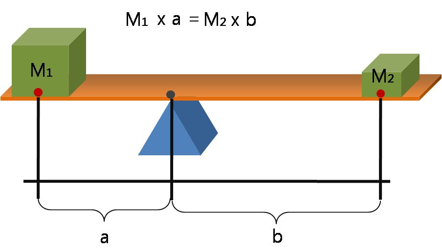
Lever Principle 3D, Jjw, CC BY-SA 3.0 https://creativecommons.org/licenses/by-sa/3.0, via Wikimedia Commons
We can find the Markov inequality from playing a game with a seesaw. The game is as follows:

gold coin Markov inequality game, Fabien Bryans, This work is licensed under CC BY-NC-SA 4.0 https://creativecommons.org/licenses/by-nc-sa/4.0/
-
You are given 1000 identical small gold coins.
-
I will give you 2 non-negative values A and B, where A < B. You are also given a seesaw of no mass which has a pivot of distance A units from the left end, the distance to the right end is effectively infinite (although remember it doesn’t weight anything).
-
You may place the coins anywhere along the seesaw.
-
You score 1 point for every gold coin placed on the seesaw at a distance equal to or further than B units from the left end.
-
Once you have placed the final coin, you only score any points if and only if the seesaw is balanced, or rotates anti-clockwise (e.g. you get a score of 0 if it rotates clockwise).
-
You win the game if you come up with an algorithm which for whatever values of A and B I give it, it describes where to place each of the 1000 coins to maximise the score for those A and B values.
How would you go about playing this game? What algorithm would you come up with?
Take some time to actually try and play the game and figure out a strategy!
Ok, so here is how you might go about thinking about it. You basically have two responsibilities in this game. Firstly, ensure that the seesaw never rotates clockwise. Secondly, get as many gold coins on or past B as possible. Logically, for every coin you put on the right hand side of the pivot you will need to put another coin the same distance from the pivot on the left hand side to keep the seesaw balanced. Alternatively, you could put 2 gold coins on the right a distance x from the pivot and 1 gold coin to counter balance a distance 2x left of the pivot. This might motivate to us that we want to maximise the distance from the pivot on the left side of the pivot in order to maximise the leverage and anti-clockwise moment. It’s also worth noting that there is no point putting a gold coin on the right side of the pivot if it doesn’t cross the B mark, as it will only contribute to the clockwise moment without scoring us a point. There is also no point in putting a gold coin any further to the right than the B mark as it will not score us any extra points but it will increase the clockwise moment. Therefore, the optimal way to score points is to have a certain proportion of the 1000 coins on the B mark, and the rest of the coins on the far left hand side of the seesaw.

gold coin Markov inequality game example, Fabien Bryans, This work is licensed under CC BY-NC-SA 4.0 https://creativecommons.org/licenses/by-nc-sa/4.0/
How do we determine what proportion of the 1000 coins should be placed on the right side? Well, we need to ensure it is balanced or atleast rotates anti-clockwise so we need the moment on the left of the pivot to be greater than or equal to the moment on the right. We can therefore form the equation:
$$(1000 - n) \times A \geq n \times (B-A)$$
Where n is the number of coins on the right hand side.
We can solve this to find n:
$$ \begin{align} 1000A - nA &\geq nB - nA \nonumber \\ 1000A &\geq nB \nonumber \\ \frac{1000A}{B} &\geq n \nonumber \\ \end{align} $$Therefore, to maximise our score, we need to maximise n, so the best score we can get is rounding down to the nearest integer of 1000A/B. We also have an algorithm for how to place the coins which is to place n of them at B, and 1000-n at the far left end of the pivot. Let’s test our algorithm on an example; A = 65, and B = 80.
$$ \begin{align} n &\leq \frac{65,000}{80} \nonumber \\ n &\leq 812.5 \nonumber \\ n &= 812 \nonumber \\ \end{align} $$So we place about 81% of the coins on the B mark and about 19% on the far left… This is the same as our result for using the Markov inequality on the baguettes!
There are a couple reasons for this. Firstly, we can view the mean of a distribution to be the “balancing point/pivot” for the moments of the data points (where instead of mass you have the probability of that value). This is therefore how we encode the information about the mean of the distribution into the problem. Secondly, the Markov inequality gives us the bound for the distribution which maximises the amount of “probability” past a point whilst still preserving the mean constraint. What we have done with the seesaw game is find this distribution, just instead of maximising “probability” we maximise “precentage of coins” - which hopefully you can see maps onto probabiliy.
So here is the Markov inequality again. Hopefully it should feel much more intuitive now when you look at it :)
$$P(X \geq a) \leq \frac{E(X)}{a}$$
a maps to B in our seesaw game, and E(X) maps to A.
Further thoughts
There are many interesting probability bounds and inequalities, the most commonly used are probably Jensen’s inequality and Chebyshev’s inequality, but many other’s can be found in this list.
I came up with this intuition for the Markov inequality independently, but after looking online I found out someone else had of course thought of it before me. The intuition is also mentioned in Berkeley’s CS70 Discrete Mathematics and Probability Theory course in Lecture 18 on Chebyshev’s inequality.