The tri-spine horseshoe crab

Recently I saw the wildlife photographer of the year competition at the natural history museum. It was cool to see lots of amazing photos! The overall winning photo of the competition was a picture of a tri-spine horseshoe crab.

When looking at the photo I noticed the pattern on the shell. Its very interesting to look at. You can follow a black line and it seems like there is always a path which goes on forever, but sometimes you can find lines which are like “islands” as you can easily see they have no loops and all paths become dead ends. The general pattern which emerges looks somewhat hexaganol, however looking closely you see these gaps are usually not hexagonal and are usually not equally sized. I wondered then, how are these patterns formed?

I had a look on google and unfortunately I couldn’t find any article or paper which looks into why this pattern forms. I did find out about Turing patterns. Turing patterns are patterns formed by diffusion and reactions of particles. Stripes, dots, spirals, hexagons, and more complex patterns can all be created by Turing patterns and so I wondered if I could create a Turing pattern simulation which generates a pattern similar to the pattern on the tri-spine horseshoe crab.

Turing patterns

How do they work?

Turing patterns were discovered by Alan Turing, who theorised that simple patterns in nature could arise simply through a reaction-diffusion system. A basic setup for this is to consider 2 chemicals, u and v. Where if u and v react with each other as follows:

$$ \begin{align} \frac{du}{dt} &= f(u, v) \nonumber \\ \frac{dv}{dt} &= g(u, v) \nonumber \\ \end{align} $$

Then we can model the system as:

$$ \begin{align} \frac{\partial u}{\partial t} &= D_{u}\nabla ^{2} u + f(u, v) \nonumber \\ \frac{\partial v}{\partial t} &= D_{v}\nabla ^ {2} v + g(u, v) \nonumber \\ \end{align} $$

Where D refers to a diffusion coefficient for a chemical.

The squared upside down triangle symbol is the Laplacian. It gives the divergence of the gradient - which is to say it gives the sum of the rate of change of the rate of change around a point. It is therefore defined as the sum of the second derivatives of each parameter. It is used here to model the diffusion of a chemical as it will give the rate of change of the concentration of the chemical. This rate of change of diffusion is also given a constant coefficient, D, to control the speed at which that chemcial diffuses.

This is basically the form of any Turing pattern. There exist many different models based on this baseline, some models include more than 2 chemicals or some will include a complicated chemical reaction function. A fairly simple model I will use will be the Gray-Scott model.

The Gray-Scott Model

The Gray-Scott model is a 2 chemical reaction-diffusion model. The reaction uses up chemical u to create chemical v.

$$U + 2V \rightarrow 3V$$

The model introduces u and removes v with time. The rate for introducing u is determined by the feed rate, f. The rate for removing v is determined by the kill rate, k. This gives us the complete model:

$$ \begin{align} \frac{\partial u}{\partial t} &= D_{u}\nabla ^{2} u - uv^{2} + f(1 - u) \nonumber \\ \frac{\partial v}{\partial t} &= D_{v}\nabla ^ {2} v + uv^{2} - (f + k) v \nonumber \\ \end{align} $$

Where u and v are between 0 and 1.

To implement this, we will be using a finite grid which will hold concentrations of u and v particles at each point in the grid. The equations are fairly simple to implement, the only thing which is non-obvious is the Laplacian. How do we implement this for a discretised 2d grid? To figure this out its worth remembering that the Laplacian is the sum of second derivatives for all parameters - for a grid this could be x and y coordinates. For the x parameter you would therefore just find the rate of change on either side of the pixel you are looking at, and then calculate the changes of these rates of change. You should then do the same for the y parameter.

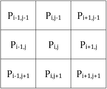
This would give us:

$$ \begin{align} \frac{\partial^{2} P}{\partial x^{2}} &= \frac{1}{\epsilon}(\frac{1}{\epsilon}(P_{i-1, j} - P_{i, j}) - \frac{1}{\epsilon}(P_{i, j} - P_{i+1, j})) \nonumber \\ &= \frac{1}{\epsilon^{2}}(P_{i-1, j} - 2 P_{i, j} + P_{i+1, j}) \nonumber \\ \frac{\partial^{2} P}{\partial y^{2}} &= \frac{1}{\epsilon}(\frac{1}{\epsilon}(P_{i, j-1} - P_{i, j}) - \frac{1}{\epsilon}(P_{i, j} - P_{i, j+1})) \nonumber \\ &= \frac{1}{\epsilon^{2}}(P_{i, j-1} - 2 P_{i, j} + P_{i, j+1}) \nonumber \\ \frac{\partial^{2} P}{\partial x^{2}} + \frac{\partial^{2} P}{\partial y^{2}} &= \frac{1}{\epsilon^{2}} (P_{i-1, j} + P_{i+1, j} + P_{i, j-1} + P_{i, j+1} - 4 P_{i, j}) \nonumber \\ \end{align} $$

We can turn this into a matrix we can convolve across the surface to give the Laplacian at each point:

$$ \begin{bmatrix} 0 & 1 & 0 \\ 1 & -4 & 1 \\ 0 & 1 & 0 \end{bmatrix} $$

We could alternatively use a slightly more detailed matrix derived using the same ideas. For example:

$$ \begin{bmatrix} 1 & 4 & 1 \\ 4 & -20 & 4 \\ 1 & 4 & 1 \end{bmatrix} $$

Coded model

Firstly, I create some helper functions to: create an empty surface and plot a surface.

# create surface
def create_empty_surface(size: int) -> np.ndarray:
  return np.zeros((2, size, size))

# plot surface
def plot_surface(surface: np.ndarray, cmap: str ="PiYG", plot: bool =False) -> np.ndarray:
  N = len(surface[0, 0])
  plot_surface = create_empty_surface(N)[0]
  plot_surface = (surface[0] / (surface[0] + surface[1]))
  plot_surface = np.where(np.isnan(plot_surface), 0.5, plot_surface)
  if plot:
    plt.imshow(plot_surface, cmap=cmap, vmin=0, vmax=1)
  return plot_surface

Next, I define the Gray-Scott model and implement a method to perform a simulation step.

class gray_scott_model:
  def __init__(self, 
            diffuse_matrix: np.ndarray, 
            diffuse_A_rate: float, 
            diffuse_B_rate: float, 
            kill_rate: float, 
            feed_rate: float, 
            starting_surface: np.ndarray =None, 
            N: int =101):
    if diffuse_matrix.sum() != 0:
      raise Exception(f"diffuse_matrix elements must sum to 0. They instead sum to {diffuse_matrix.sum()}")
    if diffuse_matrix.shape != (3, 3):
      raise Exception(f"diffuse_matrix must be of shape (3, 3). Shape is instead {diffuse_matrix.shape}")
    if diffuse_A_rate > 1 or diffuse_A_rate < 0:
      raise Exception(f"diffuse_A_rate must be between 0 and 1 inclusive, it is instead {diffuse_A_rate}")
    if diffuse_B_rate > 1 or diffuse_B_rate < 0:
      raise Exception(f"diffuse_B_rate must be between 0 and 1 inclusive, it is instead {diffuse_B_rate}")
    if kill_rate >= 1 or kill_rate <= 0:
      raise Exception(f"kill_rate must be between 0 and 1 not inclusive, it is instead {kill_rate}")
    if feed_rate >= 1 or feed_rate <= 0:
      raise Exception(f"feed_rate must be between 0 and 1 not inclusive, it is instead {feed_rate}")

    if starting_surface is None:
      starting_surface = create_empty_surface(N)
      starting_surface[0] = starting_surface[0] + 1
      starting_surface[1] = starting_surface[1] + 0
      middle_square_size = 10
      starting_surface[1][int(N/2) - int(middle_square_size/2) : int(N/2) + int(middle_square_size/2) + 1, 
                          int(N/2) - int(middle_square_size/2) : int(N/2) + int(middle_square_size/2) + 1] = 1
    
    self.diffuse_matrix = diffuse_matrix
    self.diffuse_A_rate = diffuse_A_rate
    self.diffuse_B_rate = diffuse_B_rate
    self.kill_rate = kill_rate
    self.feed_rate = feed_rate
    self.surface = starting_surface

  def simulate_step(self) -> np.ndarray:
    A = self.surface[0]
    B = self.surface[1]
    
    L_A = signal.convolve2d(A, self.diffuse_matrix, mode='same', boundary='fill', fillvalue=0)
    L_B = signal.convolve2d(B, self.diffuse_matrix, mode='same', boundary='fill', fillvalue=0)

    new_surface = create_empty_surface(len(self.surface[0, 0]))
    new_surface[0] = A + self.diffuse_A_rate*L_A - A*B*B + self.feed_rate*(1-A)
    new_surface[1] = B + self.diffuse_B_rate*L_B + A*B*B - self.kill_rate*B
    self.surface = np.clip(new_surface, a_min=0, a_max=1)
    
    return self.surface

Calibrating the constants to a known example, I find that my model produces an identical pattern which validates that the model has been implemented correctly.

Playing around with parameters I find that I can reproduce many types of patterns.

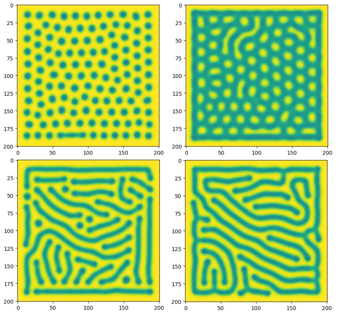
Unfortunately, despite playing around a lot, I cannot get something which closely resembles the pattern on the shell of the horseshoe crab. Looking online I found a resource which displays the produced Turing patterns over the search of the f and k parameter space. It’s cool to be able to visualise this space, but unfortunately there appears to be no pattern similar to the crab’s shell pattern. This is not too surprising. For a start, I was looking only at the Gray-Scott model. I chose this model based on trying to create Turing patterns, not because I saw biological or chemical evidence for it being an accurate model of the shell. A more representative model may have multiple chemicals, many eligible reactions, parameters as functions of time, external physical influcences, etc. Truthfully, the specifics of the chemical reactions in the shell are currently unknown and so it is probably better to do biological/chemical research into the creatures and shells in order to create a model which fits the pattern. This approach would be much better than trial and error as not only do I think it would be quicker to get to an accurate model, but also it would provide genuine insight and explainability towards interesting questions such as why specifically this pattern and why does it form.

Further thoughts and resources

I thought I might be able to derive a simulation to recreate the pattern by learning more about the production of the shell. Unfortunately there is limited literature about these creatures, and only a couple papers on their shells ^{1 2}. These papers do go into more depth about the structure of the layers which make up the shell, however the details of these papers are a bit beyond me or inaccessible to me. What I could confidently determine is that the shell is made of a protein called Chitin and an adult crab will molt about once a year. Originally I assumed the pattern must be from a chemical reaction, however it may instead come from the process of growing the shell under the current shell before molting. I tried to look a bit into mathematics for shell formation, and although there is a lot of maths trying to model shell growth, it seems like this might go into far more complexity than I feel I can look at. Regardless, it may be another possible explanation for how the pattern forms.

For learning more about Turing patterns, I can recommend Phillip Compeau’s Biological Modeling online course which walks through Turing patterns nicely. I can also recommend the “Physics for the Birds” youtube video on tiger skin cake and how Turing patterns might form it. Unrelated to Turing patterns, but I’d also recommend checking out the other photos from the wildlife photographer of the year competition :)