What is object detection?
Object detection is a type of computer vision where a system is given a list of objects it needs to identify, and then for each image it must identify any instance of one of the objects. This means it needs to return a list of bounding boxes which cover these objects and a label for each box. Object detection is used in many industries, and is usually an important tool for robotics systems to navigate and interact with their environment.
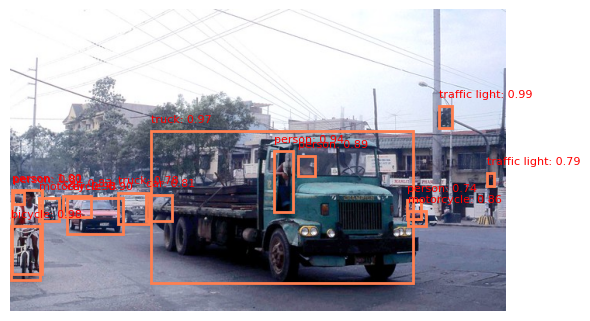
Adapted image from COCO dataset, image ID 468405
If object detection is being used in real time, then it is important that the object detection algorithm runs quickly. A slow algorithm runs the risk of having a system react based on an environment view which is no longer recent enough to apply - imagine trying to catch a ball if your vision had a 1 second delay. Another benefit of a faster algorithm is that it can evaluate more frames a second meaning that you have more data to make better inferences on motion of objects.
Faster R-CNN
The Faster R-CNN algorithm is a neural network architecture for object detection. R-CNNs (Region-based Convolutional Neural Networks) were introduced in 2014 and were an early approach to use CNNs for object detection. A year later, a faster version called the Fast R-CNN was introduced, and then the same year the Faster R-CNN was created. The main improvement of the Faster R-CNN was the usage of a region proposal network (RPN) which cuts down on the amount of regions needed to be checked by the fully connected classification and regression layers. This leads to much faster inference for an image.
Architecture overview

Figure 3. Architecture of faster region-based convolutional neural network (Faster R-CNN) , Choi et al. “Faster Region-Based Convolutional Neural Network in the Classification of Different Parkinsonism Patterns of the Striatum”, Expert Review of Molecular Diagnostics 11 (2021)
The faster R-CNN architecture consists of 3 main parts:
- A backbone network
- A region proposal network
- classification and regression networks
Backbone network
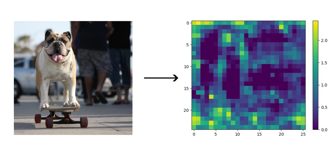
Adapted image from COCO dataset (using pretrained ResNet50 faster R-CNN, slice 1337), image ID 441470
The first stage of the faster R-CNN is the backbone network. This is a network which transforms the input image into a smaller, feature-rich form. A common way to do this is to use a convolutional network such as a VGG or ResNet model. You can even use pretrained models for this and use transfer learning to finetune these models to the specific problem domain which would cut down on training time compared to training the models from scratch.
The aim of the backbone network is to get the image into a smaller, more feature-rich form so that we can efficiently search it for any regions of interest. As the new form is smaller it means that we can exhaustively search this form whereas the original input would have been too large and time consuming to exhaustively search. Additionally, as the new form is already partly processed, it means that we can use a classifier with less parameters to determine if an area is of interest; making inference much faster.
Region proposal network
The region proposal network (RPN) uses the feature map (the output of the backbone network) to generate a set of region proposals which are more likely to have an object of interest in. Importantly, the region proposal network shouldn’t worry too much about false positives, so long as it doesn’t miss any actual objects and still cuts down by orders of magnitude on the number of regions to search then it is contributing positively to the whole architecture. The RPN consists of a mechanism to split up the feature map (which are anchor boxes), a classifier to determine if a region is of interest, and a regression layer to determine how to make the bounding box a better fit.
Anchor boxes
One problem we face is that we don’t know whether objects we need to detect are large, small, wide (like a human lying down), or tall (like a human standing up). We could try and just use a single large box which we check within across the feature map, however this will risk missing smaller objects and also might have problems if 2 different objects we are trying to detect fall in the same box.
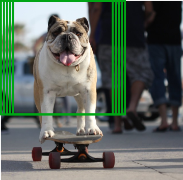
Adapted image from COCO dataset, image ID 441470
Instead, we use a set of anchor boxes which we check across our whole feature map. An anchor box set consists of a variety of scales and aspect ratios from which we check each of these created boxes for an object. See below an example of 3 scale and 3 aspect ratios for a set of anchor boxes. We then apply these anchor boxes to every point in the feature map.
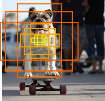
Adapted image from COCO dataset, image ID 441470
Classifier
The classifier will go through each anchor box for each point in the feature map and return a probability of there being an object in that anchor box. This is therefore a 2 class classification problem. As we assume most anchor boxes will be empty of any relevant objects, there isn’t much point in producing a probability distribution over all possible classes as most would be near 0. Therefore, we avoid using a model which may require more parameters and instead use a binary class classifier which should be faster but still classify all of the regions of interest (again, we don’t mind too much any false positives so long as the classifier still cuts down massively the number of regions we need to do a more extensive search on).
A good question here is how do we train such a network? Obviously, if we have an input to the classifier completely include an object we are looking for then it should classify it as a region of interest (ROI). Equally, if an input to the classifier includes no object at all then it should be classified as not a region of interest. But what about an input which includes most of an object? It doesn’t seem right to get the classifier to try and label this as either completely a region of interest or a region of no interest. We could just disclude any data like this from our training set on the classifier, but then what if in a production environment we catch an object halfway off the screen? In this case it would likely not be classified as a region of interest when in practice it should be. Moreover, excluding any data other than perfect data may lead the model to only classify boxes as regions of interest when there is clearly an object in them which could lead to missing out some regions (and as we do mind false negatives this is a problem). Ideally, we would be able to assign a distribution over the 2 classes for each training input, but how would we determine what the values in this distribution should be for each training input? For this we can use a heuristic called the Intersection over Union (IoU).
Intersection over Union heuristic (IoU)
The intersection over union heuristic (IoU) is a way to solve the previously mentioned problem. The metric is calculated (unsurprisingly) by calculating the area of intersection between a ground truth box and the input anchor box, and dividing this by the union of these two boxes. See the diagram below for a visual explanation.
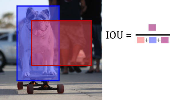
Adapted image from COCO dataset, image ID 441470
This will give a score of 0 if the anchor box and ground truth box do not intersect at all, and a value of 1 if they line up perfectly. It also gives a reasonable metric for when the boxes only align somewhat. When training the classifier, we will only give it samples where the IoU score is greater than some threshold (usually somewhere between 0.6 to 0.8, use a lower threshold if very small objects are in the training data). The selected samples will be labelled as positive for being regions of interest. We similarly will select boxes which have IoU scores less than a threshold (usually 0.1 to 0.3), to be used as negative samples for regions of interest. It’s worth noting that we only select a sample of the eligible anchor boxes to be used as training data for the classifier and regressor as otherwise training may take too long. Additionally, we sample as many positive as negative data points.
Classifier and bounding box regressor
We now have the data to do training on the RPN. The final outputs of an RPN will be a classification score if an anchor box is an area of interest or not. If it is, there will also be a regression score for how that anchor box should be adjusted so that it better fits the region of interest. The training loss for this will be given by:
$$ \begin{align*} \mathcal{L}(a, d) = \frac{1}{N_{cls}} \sum_{i} \mathcal{L}_{cls}(a_{i}, a^{*}_{i}) \ + \ \frac{\lambda}{N_{reg}} \sum_{i} \mathcal{L}_{reg}(d_{i}, d^{*}_{i}) \\ \end{align*} $$Where aᵢ is the ith prediction of the anchor box being a region of interest, aᵢ is the ground truth of that anchor box being the region of interest, dᵢ is the ith anchor box’s predicted box dimension adjustments, and dᵢ is the ground truth of that anchor box’s dimension adjustments.
$N_{cls}$ is the normalisation term for the classifier and is usually set to the total number of anchor locations. $N_{reg}$ is another normalising normalisation term, but for the bounding box regression model, and is usually set to the number of positively labelled anchor locations. $\lambda$ is a balancing parameter which can be set to prioritise either tuning of the bounding boxes or better classification, it is usually set to balance the importance of the two losses.
$$ \begin{align*} \mathcal{L}_{cls}(a_{i}, a^{*}_{i}) &= -a^{*}_{i} \cdot \log a_{i} - (1 - a^{*}_{i}) \log (1-a_{i}) \\ \end{align*} $$As the classifier is just trying to determine if a region is a ROI or not, it means it’s a binary classification task and so we can use the logistic regression loss/binary cross-entropy loss.
$$ \begin{align*} \mathcal{L}_{reg}(d_{i}, d^{*}_{i}) &= \mathbb{1}_{a^{*}_{i} = 1} \cdot L_{\delta}(d_{i} - d^{*}_{i}) \\ \end{align*} $$We use an indicator variable here because the loss for bounding box regression should only be included if the ith anchor box actually is a ROI, otherwise it doesn’t actually matter what is outputted so long as the anchor box isn’t a ROI. $L_{\delta}$ is the Huber loss function and is a loss function which provides robust regression, improving the performance of the bounding box regressor. The function is less sensitive to outliers as it penalises them linearly, whereas when the loss is smaller than some threshold, $\delta$, it is penalised quadratically. This gives the loss function a smoothing effect and is also sort of a form of regularisation (emphasis on “sort of”).
$$ L_{\delta}(x) = \begin{cases} \frac{1}{2} x^{2} & \text{if } |x| \leq \delta\\ \delta \cdot (|x| - \frac{1}{2}\delta) & \text{otherwise} \end{cases} $$We now will have a region proposal network (RPN) which when given a feature map will output a list of bounding boxes which are regions of interest (ROI) for that feature map.
Detector
The detector receives a list of ROI bounding boxes from the RPN and also has access to the feature map. The objective of the detector is to determine which class a ROI should be classified as or if it should actually just be classified as the background. The detector will also output an improved bounding box if it is a class we are looking for.
ROI pooling
The first step is to standardise the input shape to the detector by extracting the ROIs from the feature map and perform pooling on them so they are all of the same fixed shape. It does this by first extracting the region for the feature map. It then splits this region up into a fixed sized grid, and quantises the “pixels” in the region into the squares in this grid. It then performs a pooling operation (usually max pooling) on each grid square which then outputs a ROI feature map of fixed sized regardless of the size of the inputted region.

Figure 6. Illustration of the RoI pooling operation, Liu et al. “Hierarchical Feature Aggregation from Body Parts for Misalignment Robust Person Re-Identification”, Applied Sciences 9, no. 11: 2255 (2019)
Classifier and regression
The ROI feature map is fed into a fully connected network which returns a probability distribution over all the possible output classes + 1 (the +1 is for the “background” class). The ROI feature map is also fed into another fully connected layer which returns bounding box alteration which should be made for each possible class (output of shape #classes, 4). Loss is calculated similarly to the classifier and regressor in the RPN, but with a multi class classification loss function for the classifier.
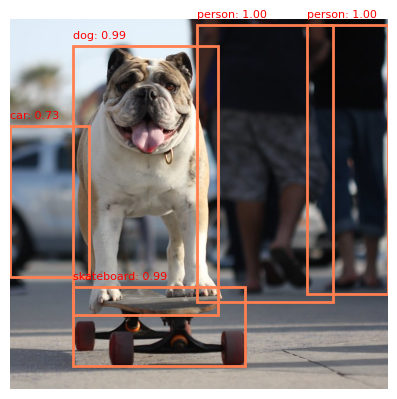
All ROIs which are classified as anything other than the background class have their proposed bounding box changes applied and are mapped back to the location on the original input image. This will therefore output a list of bounding boxes and labels which can be used with the original input image to locate and classify all instances of classes the network has been trained to identify.
Adapted image from COCO dataset, image ID 441470
PyTorch implementation
Pytorch has several faster R-CNN models. The main difference between these is the backbone network used in the architecture. These models can be loaded with pretrained parameters based on training from the COCO dataset.
torchvision.models.detection.fasterrcnn_resnet50_fpn(pretrained=True)
model architecture
FasterRCNN(
  (transform): GeneralizedRCNNTransform(
      Normalize(mean=[0.485, 0.456, 0.406], std=[0.229, 0.224, 0.225])
      Resize(min_size=(800,), max_size=1333, mode='bilinear')
  )
  (backbone): BackboneWithFPN(
    (body): IntermediateLayerGetter(
      (conv1): Conv2d(3, 64, kernel_size=(7, 7), stride=(2, 2), padding=(3, 3), bias=False)
      (bn1): FrozenBatchNorm2d(64, eps=0.0)
      (relu): ReLU(inplace=True)
      (maxpool): MaxPool2d(kernel_size=3, stride=2, padding=1, dilation=1, ceil_mode=False)
      (layer1): Sequential(
        (0): Bottleneck(
          (conv1): Conv2d(64, 64, kernel_size=(1, 1), stride=(1, 1), bias=False)
          (bn1): FrozenBatchNorm2d(64, eps=0.0)
          (conv2): Conv2d(64, 64, kernel_size=(3, 3), stride=(1, 1), padding=(1, 1), bias=False)
          (bn2): FrozenBatchNorm2d(64, eps=0.0)
          (conv3): Conv2d(64, 256, kernel_size=(1, 1), stride=(1, 1), bias=False)
          (bn3): FrozenBatchNorm2d(256, eps=0.0)
          (relu): ReLU(inplace=True)
          (downsample): Sequential(
            (0): Conv2d(64, 256, kernel_size=(1, 1), stride=(1, 1), bias=False)
            (1): FrozenBatchNorm2d(256, eps=0.0)
          )
        )
        (1): Bottleneck(
          (conv1): Conv2d(256, 64, kernel_size=(1, 1), stride=(1, 1), bias=False)
          (bn1): FrozenBatchNorm2d(64, eps=0.0)
          (conv2): Conv2d(64, 64, kernel_size=(3, 3), stride=(1, 1), padding=(1, 1), bias=False)
          (bn2): FrozenBatchNorm2d(64, eps=0.0)
          (conv3): Conv2d(64, 256, kernel_size=(1, 1), stride=(1, 1), bias=False)
          (bn3): FrozenBatchNorm2d(256, eps=0.0)
          (relu): ReLU(inplace=True)
        )
        (2): Bottleneck(
          (conv1): Conv2d(256, 64, kernel_size=(1, 1), stride=(1, 1), bias=False)
          (bn1): FrozenBatchNorm2d(64, eps=0.0)
          (conv2): Conv2d(64, 64, kernel_size=(3, 3), stride=(1, 1), padding=(1, 1), bias=False)
          (bn2): FrozenBatchNorm2d(64, eps=0.0)
          (conv3): Conv2d(64, 256, kernel_size=(1, 1), stride=(1, 1), bias=False)
          (bn3): FrozenBatchNorm2d(256, eps=0.0)
          (relu): ReLU(inplace=True)
        )
      )
      (layer2): Sequential(
        (0): Bottleneck(
          (conv1): Conv2d(256, 128, kernel_size=(1, 1), stride=(1, 1), bias=False)
          (bn1): FrozenBatchNorm2d(128, eps=0.0)
          (conv2): Conv2d(128, 128, kernel_size=(3, 3), stride=(2, 2), padding=(1, 1), bias=False)
          (bn2): FrozenBatchNorm2d(128, eps=0.0)
          (conv3): Conv2d(128, 512, kernel_size=(1, 1), stride=(1, 1), bias=False)
          (bn3): FrozenBatchNorm2d(512, eps=0.0)
          (relu): ReLU(inplace=True)
          (downsample): Sequential(
            (0): Conv2d(256, 512, kernel_size=(1, 1), stride=(2, 2), bias=False)
            (1): FrozenBatchNorm2d(512, eps=0.0)
          )
        )
        (1): Bottleneck(
          (conv1): Conv2d(512, 128, kernel_size=(1, 1), stride=(1, 1), bias=False)
          (bn1): FrozenBatchNorm2d(128, eps=0.0)
          (conv2): Conv2d(128, 128, kernel_size=(3, 3), stride=(1, 1), padding=(1, 1), bias=False)
          (bn2): FrozenBatchNorm2d(128, eps=0.0)
          (conv3): Conv2d(128, 512, kernel_size=(1, 1), stride=(1, 1), bias=False)
          (bn3): FrozenBatchNorm2d(512, eps=0.0)
          (relu): ReLU(inplace=True)
        )
        (2): Bottleneck(
          (conv1): Conv2d(512, 128, kernel_size=(1, 1), stride=(1, 1), bias=False)
          (bn1): FrozenBatchNorm2d(128, eps=0.0)
          (conv2): Conv2d(128, 128, kernel_size=(3, 3), stride=(1, 1), padding=(1, 1), bias=False)
          (bn2): FrozenBatchNorm2d(128, eps=0.0)
          (conv3): Conv2d(128, 512, kernel_size=(1, 1), stride=(1, 1), bias=False)
          (bn3): FrozenBatchNorm2d(512, eps=0.0)
          (relu): ReLU(inplace=True)
        )
        (3): Bottleneck(
          (conv1): Conv2d(512, 128, kernel_size=(1, 1), stride=(1, 1), bias=False)
          (bn1): FrozenBatchNorm2d(128, eps=0.0)
          (conv2): Conv2d(128, 128, kernel_size=(3, 3), stride=(1, 1), padding=(1, 1), bias=False)
          (bn2): FrozenBatchNorm2d(128, eps=0.0)
          (conv3): Conv2d(128, 512, kernel_size=(1, 1), stride=(1, 1), bias=False)
          (bn3): FrozenBatchNorm2d(512, eps=0.0)
          (relu): ReLU(inplace=True)
        )
      )
      (layer3): Sequential(
        (0): Bottleneck(
          (conv1): Conv2d(512, 256, kernel_size=(1, 1), stride=(1, 1), bias=False)
          (bn1): FrozenBatchNorm2d(256, eps=0.0)
          (conv2): Conv2d(256, 256, kernel_size=(3, 3), stride=(2, 2), padding=(1, 1), bias=False)
          (bn2): FrozenBatchNorm2d(256, eps=0.0)
          (conv3): Conv2d(256, 1024, kernel_size=(1, 1), stride=(1, 1), bias=False)
          (bn3): FrozenBatchNorm2d(1024, eps=0.0)
          (relu): ReLU(inplace=True)
          (downsample): Sequential(
            (0): Conv2d(512, 1024, kernel_size=(1, 1), stride=(2, 2), bias=False)
            (1): FrozenBatchNorm2d(1024, eps=0.0)
          )
        )
        (1): Bottleneck(
          (conv1): Conv2d(1024, 256, kernel_size=(1, 1), stride=(1, 1), bias=False)
          (bn1): FrozenBatchNorm2d(256, eps=0.0)
          (conv2): Conv2d(256, 256, kernel_size=(3, 3), stride=(1, 1), padding=(1, 1), bias=False)
          (bn2): FrozenBatchNorm2d(256, eps=0.0)
          (conv3): Conv2d(256, 1024, kernel_size=(1, 1), stride=(1, 1), bias=False)
          (bn3): FrozenBatchNorm2d(1024, eps=0.0)
          (relu): ReLU(inplace=True)
        )
        (2): Bottleneck(
          (conv1): Conv2d(1024, 256, kernel_size=(1, 1), stride=(1, 1), bias=False)
          (bn1): FrozenBatchNorm2d(256, eps=0.0)
          (conv2): Conv2d(256, 256, kernel_size=(3, 3), stride=(1, 1), padding=(1, 1), bias=False)
          (bn2): FrozenBatchNorm2d(256, eps=0.0)
          (conv3): Conv2d(256, 1024, kernel_size=(1, 1), stride=(1, 1), bias=False)
          (bn3): FrozenBatchNorm2d(1024, eps=0.0)
          (relu): ReLU(inplace=True)
        )
        (3): Bottleneck(
          (conv1): Conv2d(1024, 256, kernel_size=(1, 1), stride=(1, 1), bias=False)
          (bn1): FrozenBatchNorm2d(256, eps=0.0)
          (conv2): Conv2d(256, 256, kernel_size=(3, 3), stride=(1, 1), padding=(1, 1), bias=False)
          (bn2): FrozenBatchNorm2d(256, eps=0.0)
          (conv3): Conv2d(256, 1024, kernel_size=(1, 1), stride=(1, 1), bias=False)
          (bn3): FrozenBatchNorm2d(1024, eps=0.0)
          (relu): ReLU(inplace=True)
        )
        (4): Bottleneck(
          (conv1): Conv2d(1024, 256, kernel_size=(1, 1), stride=(1, 1), bias=False)
          (bn1): FrozenBatchNorm2d(256, eps=0.0)
          (conv2): Conv2d(256, 256, kernel_size=(3, 3), stride=(1, 1), padding=(1, 1), bias=False)
          (bn2): FrozenBatchNorm2d(256, eps=0.0)
          (conv3): Conv2d(256, 1024, kernel_size=(1, 1), stride=(1, 1), bias=False)
          (bn3): FrozenBatchNorm2d(1024, eps=0.0)
          (relu): ReLU(inplace=True)
        )
        (5): Bottleneck(
          (conv1): Conv2d(1024, 256, kernel_size=(1, 1), stride=(1, 1), bias=False)
          (bn1): FrozenBatchNorm2d(256, eps=0.0)
          (conv2): Conv2d(256, 256, kernel_size=(3, 3), stride=(1, 1), padding=(1, 1), bias=False)
          (bn2): FrozenBatchNorm2d(256, eps=0.0)
          (conv3): Conv2d(256, 1024, kernel_size=(1, 1), stride=(1, 1), bias=False)
          (bn3): FrozenBatchNorm2d(1024, eps=0.0)
          (relu): ReLU(inplace=True)
        )
      )
      (layer4): Sequential(
        (0): Bottleneck(
          (conv1): Conv2d(1024, 512, kernel_size=(1, 1), stride=(1, 1), bias=False)
          (bn1): FrozenBatchNorm2d(512, eps=0.0)
          (conv2): Conv2d(512, 512, kernel_size=(3, 3), stride=(2, 2), padding=(1, 1), bias=False)
          (bn2): FrozenBatchNorm2d(512, eps=0.0)
          (conv3): Conv2d(512, 2048, kernel_size=(1, 1), stride=(1, 1), bias=False)
          (bn3): FrozenBatchNorm2d(2048, eps=0.0)
          (relu): ReLU(inplace=True)
          (downsample): Sequential(
            (0): Conv2d(1024, 2048, kernel_size=(1, 1), stride=(2, 2), bias=False)
            (1): FrozenBatchNorm2d(2048, eps=0.0)
          )
        )
        (1): Bottleneck(
          (conv1): Conv2d(2048, 512, kernel_size=(1, 1), stride=(1, 1), bias=False)
          (bn1): FrozenBatchNorm2d(512, eps=0.0)
          (conv2): Conv2d(512, 512, kernel_size=(3, 3), stride=(1, 1), padding=(1, 1), bias=False)
          (bn2): FrozenBatchNorm2d(512, eps=0.0)
          (conv3): Conv2d(512, 2048, kernel_size=(1, 1), stride=(1, 1), bias=False)
          (bn3): FrozenBatchNorm2d(2048, eps=0.0)
          (relu): ReLU(inplace=True)
        )
        (2): Bottleneck(
          (conv1): Conv2d(2048, 512, kernel_size=(1, 1), stride=(1, 1), bias=False)
          (bn1): FrozenBatchNorm2d(512, eps=0.0)
          (conv2): Conv2d(512, 512, kernel_size=(3, 3), stride=(1, 1), padding=(1, 1), bias=False)
          (bn2): FrozenBatchNorm2d(512, eps=0.0)
          (conv3): Conv2d(512, 2048, kernel_size=(1, 1), stride=(1, 1), bias=False)
          (bn3): FrozenBatchNorm2d(2048, eps=0.0)
          (relu): ReLU(inplace=True)
        )
      )
    )
    (fpn): FeaturePyramidNetwork(
      (inner_blocks): ModuleList(
        (0): Conv2dNormActivation(
          (0): Conv2d(256, 256, kernel_size=(1, 1), stride=(1, 1))
        )
        (1): Conv2dNormActivation(
          (0): Conv2d(512, 256, kernel_size=(1, 1), stride=(1, 1))
        )
        (2): Conv2dNormActivation(
          (0): Conv2d(1024, 256, kernel_size=(1, 1), stride=(1, 1))
        )
        (3): Conv2dNormActivation(
          (0): Conv2d(2048, 256, kernel_size=(1, 1), stride=(1, 1))
        )
      )
      (layer_blocks): ModuleList(
        (0-3): 4 x Conv2dNormActivation(
          (0): Conv2d(256, 256, kernel_size=(3, 3), stride=(1, 1), padding=(1, 1))
        )
      )
      (extra_blocks): LastLevelMaxPool()
    )
  )
  (rpn): RegionProposalNetwork(
    (anchor_generator): AnchorGenerator()
    (head): RPNHead(
      (conv): Sequential(
        (0): Conv2dNormActivation(
          (0): Conv2d(256, 256, kernel_size=(3, 3), stride=(1, 1), padding=(1, 1))
          (1): ReLU(inplace=True)
        )
      )
      (cls_logits): Conv2d(256, 3, kernel_size=(1, 1), stride=(1, 1))
      (bbox_pred): Conv2d(256, 12, kernel_size=(1, 1), stride=(1, 1))
    )
  )
  (roi_heads): RoIHeads(
    (box_roi_pool): MultiScaleRoIAlign(featmap_names=['0', '1', '2', '3'], output_size=(7, 7), sampling_ratio=2)
    (box_head): TwoMLPHead(
      (fc6): Linear(in_features=12544, out_features=1024, bias=True)
      (fc7): Linear(in_features=1024, out_features=1024, bias=True)
    )
    (box_predictor): FastRCNNPredictor(
      (cls_score): Linear(in_features=1024, out_features=91, bias=True)
      (bbox_pred): Linear(in_features=1024, out_features=364, bias=True)
    )
  )
)
Further resources
To read some of the foundational papers in the development of the faster R-CNN, you can check out “Rich feature hierarchies for accurate object detection and semantic segmentation” (Girshick et al. 2014), “Fast R-CNN” (Girshick 2015), and “Faster R-CNN: Towards Real-Time Object Detection with Region Proposal Networks” (Ren et al. 2015).
For some further helpful resources and articles on these R-CNN based models check out: “Faster R-CNN for object detection - A technical paper summary” by Shilpa Ananth, and “Object Detection for Dummies Part 3: R-CNN Family” by Lilian Weng.
To learn about YOLO, a model which also performs object detection but with much faster inference, you can read the paper “You Only Look Once: Unified, Real-Time Object Detection” (Redmon et al. 2015). To learn about how the faster R-CNN was adapted to perform image segmentation, you can read the paper “Mask R-CNN” (He et al. 2017).